Equivalent concepts in ClickStack and Elastic

Elastic Stack vs ClickStack

Both Elastic Stack and ClickStack cover the core roles of an observability platform, but they approach these roles with different design philosophies. These roles include:

• UI and Alerting: Tools for querying data, building dashboards, and managing alerts.
• Storage and Query Engine: The backend systems responsible for storing observability data and serving analytical queries.
• Data Collection and ETL: Agents and pipelines that gather telemetry data and process it before ingestion.

The table below outlines how each stack maps its components to these roles:

Role	Elastic Stack	ClickStack	Comments
UI & Alerting	Kibana — dashboards, search, and alerts	HyperDX — real-time UI, search, and alerts	Both serve as the primary interface for users, including visualizations and alert management. HyperDX is purpose-built for observability and tightly coupled to OpenTelemetry semantics.
Storage & Query Engine	Elasticsearch — JSON document store with inverted index	ClickHouse — column-oriented database with vectorized engine	Elasticsearch uses an inverted index optimized for search; ClickHouse uses columnar storage and SQL for high-speed analytics over structured and semi-structured data.
Data Collection	Elastic Agent, Beats (e.g. Filebeat, Metricbeat)	OpenTelemetry Collector (edge + gateway)	Elastic supports custom shippers and a unified agent managed by Fleet. ClickStack relies on OpenTelemetry, allowing vendor-neutral data collection and processing.
Instrumentation SDKs	Elastic APM agents (proprietary)	OpenTelemetry SDKs (distributed by ClickStack)	Elastic SDKs are tied to the Elastic stack. ClickStack builds on OpenTelemetry SDKs for logs, metrics, and traces in major languages.
ETL / Data Processing	Logstash, ingest pipelines	OpenTelemetry Collector + ClickHouse materialized views	Elastic uses ingest pipelines and Logstash for transformation. ClickStack shifts compute to insert time via materialized views and OTel collector processors, which transform data efficiently and incrementally.
Architecture Philosophy	Vertically integrated, proprietary agents and formats	Open standard–based, loosely coupled components	Elastic builds a tightly integrated ecosystem. ClickStack emphasizes modularity and standards (OpenTelemetry, SQL, object storage) for flexibility and cost-efficiency.

ClickStack emphasizes open standards and interoperability, being fully OpenTelemetry-native from collection to UI. In contrast, Elastic provides a tightly coupled but more vertically integrated ecosystem with proprietary agents and formats.

Given that Elasticsearch and ClickHouse are the core engines responsible for data storage, processing, and querying in their respective stacks, understanding how they differ is essential. These systems underpin the performance, scalability, and flexibility of the entire observability architecture. The following section explores the key differences between Elasticsearch and ClickHouse - including how they model data, handle ingestion, execute queries, and manage storage.

Elasticsearch vs ClickHouse

ClickHouse and Elasticsearch organize and query data using different underlying models, but many core concepts serve similar purposes. This section outlines key equivalences for users familiar with Elastic, mapping them to their ClickHouse counterparts. While the terminology differs, most observability workflows can be reproduced - often more efficiently - in ClickStack.

Core structural concepts

Elasticsearch	ClickHouse / SQL	Description
Field	Column	The basic unit of data, holding one or more values of a specific type. Elasticsearch fields can store primitives as well as arrays and objects. Fields can have only one type. ClickHouse also supports arrays and objects (Tuples, Maps, Nested), as well as dynamic types like Variant and Dynamic which allow a column to have multiple types.
Document	Row	A collection of fields (columns). Elasticsearch documents are more flexible by default, with new fields added dynamically based on the data (type is inferred from ). ClickHouse rows are schema-bound by default, with users needing to insert all columns for a row or subset. The JSON type in ClickHouse supports equivalent semi-structured dynamic column creation based on the inserted data.
Index	Table	The unit of query execution and storage. In both systems, queries run against indices or tables, which store rows/documents.
Implicit	Schema (SQL)	SQL schemas group tables into namespaces, often used for access control. Elasticsearch and ClickHouse don't have schemas, but both support row-and table-level security via roles and RBAC.
Cluster	Cluster / Database	Elasticsearch clusters are runtime instances that manage one or more indices. In ClickHouse, databases organize tables within a logical namespace, providing the same logical grouping as a cluster in Elasticsearch. A ClickHouse cluster is a distributed set of nodes, similar to Elasticsearch, but is decoupled and independent of the data itself.

Data modeling and flexibility

Elasticsearch is known for its schema flexibility through dynamic mappings. Fields are created as documents are ingested, and types are inferred automatically - unless a schema is specified. ClickHouse is stricter by default — tables are defined with explicit schemas — but offers flexibility through Dynamic, Variant, and JSON types. These enable ingestion of semi-structured data, with dynamic column creation and type inference similar to Elasticsearch. Similarly, the Map type allows arbitrary key-value pairs to be stored - although a single type is enforced for both the key and value.

ClickHouse's approach to type flexibility is more transparent and controlled. Unlike Elasticsearch, where type conflicts can cause ingestion errors, ClickHouse allows mixed-type data in Variant columns and supports schema evolution through the use of the JSON type.

If not using JSON, the schema is statically-defined. If values are not provided for a row, they will either be defined as Nullable (not used in ClickStack) or revert to the default value for the type e.g. empty value for String.

Ingestion and transformation

Elasticsearch uses ingest pipelines with processors (e.g., enrich, rename, grok) to transform documents before indexing. In ClickHouse, similar functionality is achieved using Incremental Materialized Views, which can filter, transform, or enrich incoming data and insert results into target tables. You can also insert data to a Null table engine if you only need the output of the materialized view to be stored. This means the only the results of any materialized views are preserved, but the original data is discarded - thus saving storage space.

For enrichment, Elasticsearch supports dedicated enrich processors to add context to documents. In ClickHouse, dictionaries can be used at both query time and ingest time to enrich rows - for example, to map IPs to locations or apply user agent lookups on insert.

Query languages

Elasticsearch supports a number of query languages including DSL, ES|QL, EQL and KQL (Lucene style) queries, but has limited support for joins — only left outer joins are available via ES|QL. ClickHouse supports full SQL syntax, including all join types, window functions, subqueries (and correlated), and CTEs. This is a major advantage for users needing to correlate between observability signals and business or infrastructure data.

In ClickStack, HyperDX provides a Lucene-compatible search interface for ease of transition, alongside full SQL support via the ClickHouse backend. This syntax is comparable to the Elastic query string syntax. For an exact comparison of this syntax, see "Searching in ClickStack and Elastic".

File formats and interfaces

Elasticsearch supports JSON (and limited CSV) ingestion. ClickHouse supports over 70 file formats, including Parquet, Protobuf, Arrow, CSV, and others — for both ingestion and export. This makes it easier to integrate with external pipelines and tools.

Both systems offer a REST API, but ClickHouse also provides a native protocol for low-latency, high-throughput interaction. The native interface supports query progress, compression, and streaming more efficiently than HTTP, and is the default for most production ingestion.

Indexing and storage

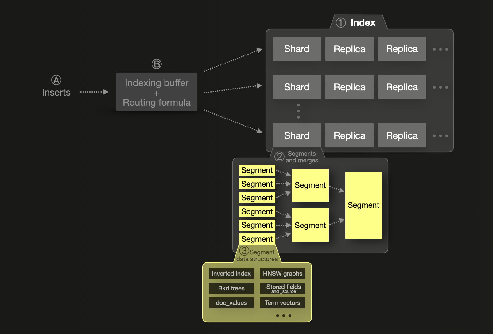
The concept of sharding is fundamental to Elasticsearch's scalability model. Each ① index is broken into shards, each of which is a physical Lucene index stored as segments on disk. A shard can have one or more physical copies called replica shards for resilience. For scalability, shards and replicas can be distributed over several nodes. A single shard ② consists of one or more immutable segments. A segment is the basic indexing structure of Lucene, the Java library providing the indexing and search features on which Elasticsearch is based.

Insert processing in Elasticsearch

Ⓐ Newly inserted documents Ⓑ first go into an in-memory indexing buffer that is flushed by default once per second. A routing formula is used to determine the target shard for flushed documents, and a new segment is written for the shard on disk. To improve query efficiency and enable the physical deletion of deleted or updated documents, segments are continuously merged in the background into larger segments until they reach a max size of 5 GB. It is possible to force a merge into larger segments, though.

Elasticsearch recommends sizing shards to around 50 GB or 200 million documents due to JVM heap and metadata overhead. There's also a hard limit of 2 billion documents per shard. Elasticsearch parallelizes queries across shards, but each shard is processed using a single thread, making over-sharding both costly and counterproductive. This inherently makes sharding tightly coupled to scaling, with more shards (and nodes) required to scale performance.

Elasticsearch indexes all fields into inverted indices for fast search, optionally using doc values for aggregations, sorting and scripted field access. Numeric and geo fields use Block K-D trees for searches on geospatial data and numeric and date ranges.

Importantly, Elasticsearch stores the full original document in _source (compressed with LZ4, Deflate or ZSTD), while ClickHouse does not store a separate document representation. Data is reconstructed from columns at query time, saving storage space. This same capability is possible for Elasticsearch using Synthetic _source, with some restrictions. Disabling of _source also has implications which don't apply to ClickHouse.

In Elasticsearch, index mappings (equivalent to table schemas in ClickHouse) control the type of fields and the data structures used for this persistence and querying.

ClickHouse, by contrast, is column-oriented — every column is stored independently but always sorted by the table's primary/ordering key. This ordering enables sparse primary indexes, which allow ClickHouse to skip over data during query execution efficiently. When queries filter by primary key fields, ClickHouse reads only the relevant parts of each column, significantly reducing disk I/O and improving performance — even without a full index on every column.

ClickHouse also supports skip indexes, which accelerate filtering by precomputing index data for selected columns. These must be explicitly defined but can significantly improve performance. Additionally, ClickHouse lets users specify compression codecs and compression algorithms per column — something Elasticsearch does not support (its compression only applies to _source JSON storage).

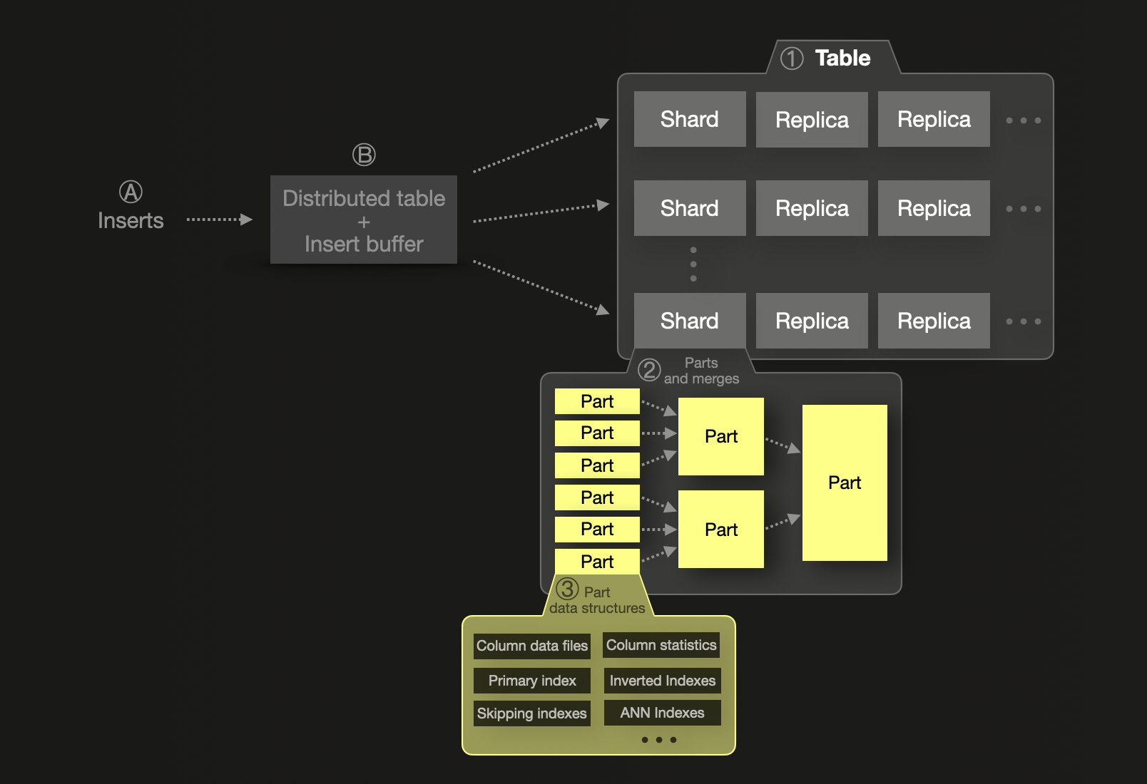
ClickHouse also supports sharding, but its model is designed to favor vertical scaling. A single shard can store trillions of rows and continues to perform efficiently as long as memory, CPU, and disk permit. Unlike Elasticsearch, there is no hard row limit per shard. Shards in ClickHouse are logical — effectively individual tables — and do not require partitioning unless the dataset exceeds the capacity of a single node. This typically occurs due to disk size constraints, with sharding ① introduced only when horizontal scale-out is necessary - reducing complexity and overhead. In this case, similar to Elasticsearch, a shard will hold a subset of the data. The data within a single shard is organized as a collection of ② immutable data parts containing ③ several data structures.

Processing within a ClickHouse shard is fully parallelized, and users are encouraged to scale vertically to avoid the network costs associated with moving data across nodes.

Insert processing in ClickHouse

ClickHouse inserts are synchronous by default — the write is acknowledged only after commit — but can be configured for asynchronous inserts to match Elastic-like buffering and batching. If asynchronous data inserts are used, Ⓐ newly inserted rows first go into an Ⓑ in-memory insert buffer that is flushed by default once every 200 milliseconds. If multiple shards are used, a distributed table is used for routing newly inserted rows to their target shard. A new part is written for the shard on disk.

Distribution and replication

While both Elasticsearch and ClickHouse use clusters, shards, and replicas to ensure scalability and fault tolerance, their models differ significantly in implementation and performance characteristics.

Elasticsearch uses a primary-secondary model for replication. When data is written to a primary shard, it is synchronously copied to one or more replicas. These replicas are themselves full shards distributed across nodes to ensure redundancy. Elasticsearch acknowledges writes only after all required replicas confirm the operation — a model that provides near sequential consistency, although dirty reads from replicas are possible before full sync. A master node coordinates the cluster, managing shard allocation, health, and leader election.

Conversely, ClickHouse employs eventual consistency by default, coordinated by Keeper - a lightweight alternative to ZooKeeper. Writes can be sent to any replica directly or via a distributed table, which automatically selects a replica. Replication is asynchronous - changes are propagated to other replicas after the write is acknowledged. For stricter guarantees, ClickHouse supports sequential consistency, where writes are acknowledged only after being committed across replicas, though this mode is rarely used due to its performance impact. Distributed tables unify access across multiple shards, forwarding SELECT queries to all shards and merging the results. For INSERT operations, they balance the load by evenly routing data across shards. ClickHouse's replication is highly flexible: any replica (a copy of a shard) can accept writes, and all changes are asynchronously synchronized to others. This architecture allows uninterrupted query serving during failures or maintenance, with resynchronization handled automatically - eliminating the need for primary-secondary enforcement at the data layer.

ClickHouse Cloud

In ClickHouse Cloud, the architecture introduces a shared-nothing compute model where a single shard is backed by object storage. This replaces traditional replica-based high availability, allowing the shard to be read and written by multiple nodes simultaneously. The separation of storage and compute enables elastic scaling without explicit replica management.

In summary:

• Elastic: Shards are physical Lucene structures tied to JVM memory. Over-sharding introduces performance penalties. Replication is synchronous and coordinated by a master node.
• ClickHouse: Shards are logical and vertically scalable, with highly efficient local execution. Replication is asynchronous (but can be sequential), and coordination is lightweight.

Ultimately, ClickHouse favors simplicity and performance at scale by minimizing the need for shard tuning while still offering strong consistency guarantees when needed.

Deduplication and routing

Elasticsearch de-duplicates documents based on their _id, routing them to shards accordingly. ClickHouse does not store a default row identifier but supports insert-time deduplication, allowing users to retry failed inserts safely. For more control, ReplacingMergeTree and other table engines enable deduplication by specific columns.

Index routing in Elasticsearch ensures specific documents and always routed to specific shards. In ClickHouse, users can define shard keys or use Distributed tables to achieve similar data locality.

Aggregations and execution model

While both systems support the aggregation of data, ClickHouse offers significantly more functions, including statistical, approximate, and specialized analytical functions.

In observability use cases, one of the most common applications for aggregations is to count how often specific log messages or events occur (and alerting in case the frequency is unusual).

The equivalent to a ClickHouse SELECT count(*) FROM ... GROUP BY ... SQL query in Elasticsearch is the terms aggregation, which is an Elasticsearch bucket aggregation.

ClickHouse's GROUP BY with a count(*) and Elasticsearch's terms aggregation are generally equivalent in terms of functionality, but they differ widely in their implementation, performance, and result quality.

This aggregation in Elasticsearch estimates results in "top-N" queries (e.g., top 10 hosts by count), when the queried data spans multiple shards. This estimation improves speed but can compromise accuracy. Users can reduce this error by inspecting doc_count_error_upper_bound and increasing the shard_size parameter — at the cost of increased memory usage and slower query performance.

Elasticsearch also requires a size setting for all bucketed aggregations — there's no way to return all unique groups without explicitly setting a limit. High-cardinality aggregations risk hitting max_buckets limits or require paginating with a composite aggregation, which is often complex and inefficient.

ClickHouse, by contrast, performs exact aggregations out of the box. Functions like count(*) return accurate results without needing configuration tweaks, making query behavior simpler and more predictable.

ClickHouse imposes no size limits. You can perform unbounded group-by queries across large datasets. If memory thresholds are exceeded, ClickHouse can spill to disk. Aggregations that group by a prefix of the primary key are especially efficient, often running with minimal memory consumption.

Execution model

The above differences can be attributed to the execution models of Elasticsearch and ClickHouse, which take fundamentally different approaches to query execution and parallelism.

ClickHouse was designed to maximize efficiency on modern hardware. By default, ClickHouse runs a SQL query with N concurrent execution lanes on a machine with N CPU cores:

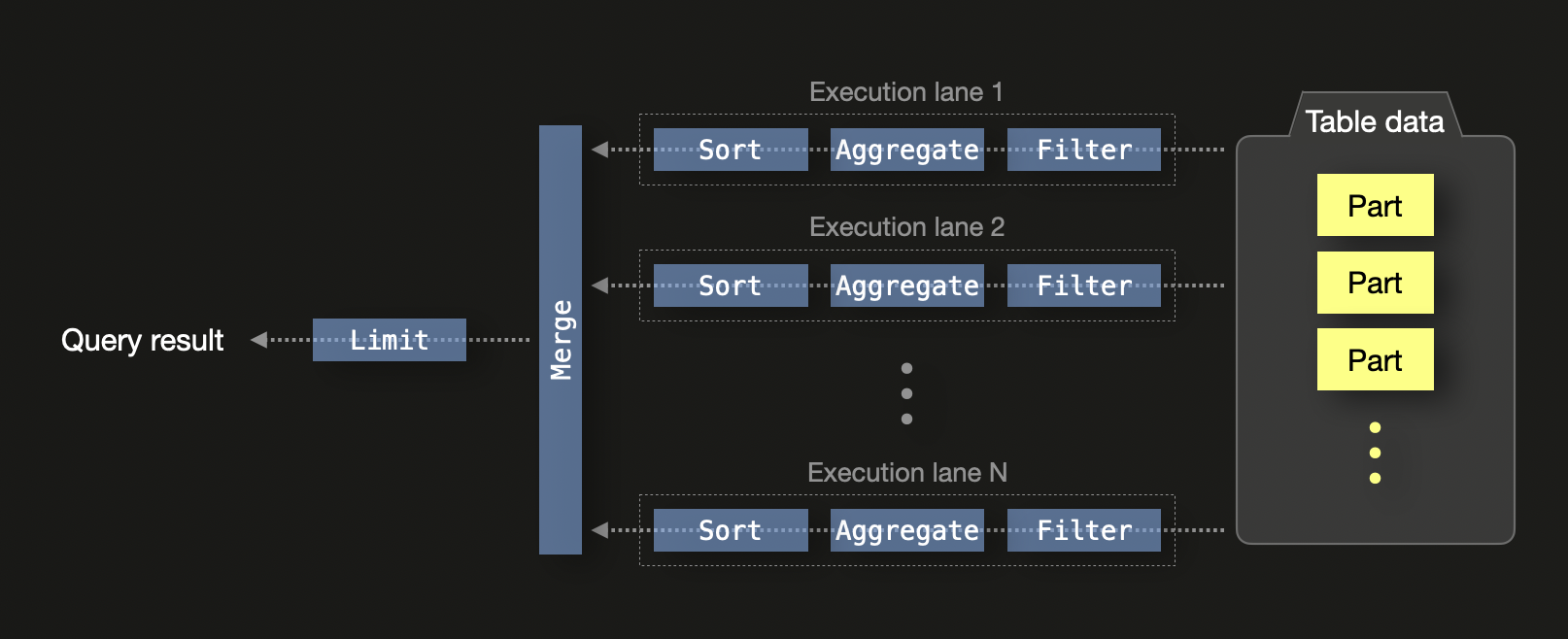
On a single node, execution lanes split data into independent ranges allowing concurrent processing across CPU threads. This includes filtering, aggregation, and sorting. The local results from each lane are eventually merged, and a limit operator is applied, in case the query features a limit clause.

Query execution is further parallelized by:

1. SIMD vectorization: Operations on columnar data use CPU SIMD instructions (e.g., AVX512), allowing batch processing of values.
2. Cluster-level parallelism: In distributed setups, each node performs query processing locally. Partial aggregation states are streamed to the initiating node and merged. If the query's GROUP BY keys align with the sharding keys, merging can be minimized or avoided entirely.

This model enables efficient scaling across cores and nodes, making ClickHouse well-suited for large-scale analytics. The use of partial aggregation states allows intermediate results from different threads and nodes to be merged without loss of accuracy.

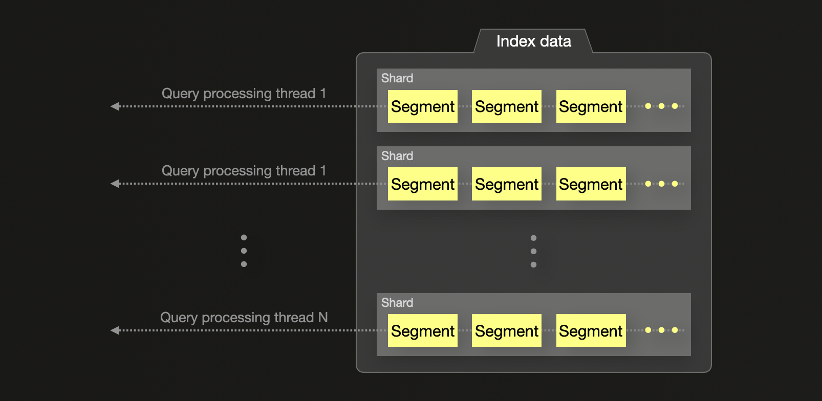
Elasticsearch, by contrast, assigns one thread per shard for most aggregations, regardless of how many CPU cores are available. These threads return shard-local top-N results, which are merged at the coordinating node. This approach can underutilize system resources and introduce potential inaccuracies in global aggregations, particularly when frequent terms are distributed across multiple shards. Accuracy can be improved by increasing the shard_size parameter, but this comes at the cost of higher memory usage and query latency.

In summary, ClickHouse executes aggregations and queries with finer-grained parallelism and greater control over hardware resources, while Elasticsearch relies on shard-based execution with more rigid constraints.

For further details on the mechanics of aggregations in the respective technologies, we recommend the blog post "ClickHouse vs. Elasticsearch: The Mechanics of Count Aggregations".

Data Management

Elasticsearch and ClickHouse take fundamentally different approaches to managing time-series observability data — particularly around data retention, rollover, and tiered storage.

Index Lifecycle Management vs Native TTL

In Elasticsearch, long-term data management is handled through Index Lifecycle Management (ILM) and Data Streams. These features allow users to define policies that govern when indices are rolled over (e.g. after reaching a certain size or age), when older indices are moved to lower-cost storage (e.g. warm or cold tiers), and when they are ultimately deleted. This is necessary because Elasticsearch does not support re-sharding, and shards cannot grow indefinitely without performance degradation. To manage shard sizes and support efficient deletion, new indices must be created periodically and old ones removed — effectively rotating data at the index level.

ClickHouse takes a different approach. Data is typically stored in a single table and managed using TTL (time-to-live) expressions at the column or partition level. Data can be partitioned by date, allowing efficient deletion without the need to create new tables or perform index rollovers. As data ages and meets the TTL condition, ClickHouse will automatically remove it — no additional infrastructure is required to manage rotation.

Storage Tiers and Hot-Warm Architectures

Elasticsearch supports hot-warm-cold-frozen storage architectures, where data is moved between storage tiers with different performance characteristics. This is typically configured through ILM and tied to node roles in the cluster.

ClickHouse supports tiered storage through native table engines like MergeTree, which can automatically move older data between different volumes (e.g., SSD to HDD to object storage) based on custom rules. This can mimic Elastic's hot-warm-cold approach — but without the complexity of managing multiple node roles or clusters.

ClickHouse Cloud

In ClickHouse Cloud, this becomes even more seamless: all data is stored on object storage (e.g. S3), and compute is decoupled. Data can remain in object storage until queried, at which point it is fetched and cached locally (or in a distributed cache) — offering the same cost profile as Elastic's frozen tier, with better performance characteristics. This approach means no data needs to be moved between storage tiers, making hot-warm architectures redundant.

Rollups vs Incremental Aggregates

In Elasticsearch, rollups or aggregates are achieved using a mechanism called transforms. These are used to summarize time-series data at fixed intervals (e.g., hourly or daily) using a sliding window model. These are configured as recurring background jobs that aggregate data from one index and write the results to a separate rollup index. This helps reduce the cost of long-range queries by avoiding repeated scans of high-cardinality raw data.

The following diagram sketches abstractly how transforms work (note that we use the blue color for all documents belonging to the same bucket for which we want to pre-calculate aggregate values):

Continuous transforms use transform checkpoints based on a configurable check interval time (transform frequency with a default value of 1 minute). In the diagram above, we assume ① a new checkpoint is created after the check interval time has elapsed. Now Elasticsearch checks for changes in the transforms' source index and detects three new blue documents (11, 12, and 13) that exist since the previous checkpoint. Therefore the source index is filtered for all existing blue documents, and, with a composite aggregation (to utilize result pagination), the aggregate values are recalculated (and the destination index is updated with a document replacing the document containing the previous aggregation values). Similarly, at ② and ③, new checkpoints are processed by checking for changes and recalculating the aggregate values from all existing documents belonging to the same 'blue' bucket.

ClickHouse takes a fundamentally different approach. Rather than re-aggregating data periodically, ClickHouse supports incremental materialized views, which transform and aggregate data at insert time. When new data is written to a source table, a materialized view executes a pre-defined SQL aggregation query on only the new inserted blocks, and writes the aggregated results to a target table.

This model is made possible by ClickHouse's support for partial aggregate states — intermediate representations of aggregation functions that can be stored and later merged. This allows users to maintain partially aggregated results that are fast to query and cheap to update. Since the aggregation happens as data arrives, there's no need to run expensive recurring jobs or re-summarize older data.

We sketch the mechanics of incremental materialized views abstractly (note that we use the blue color for all rows belonging to the same group for which we want to pre-calculate aggregate values):

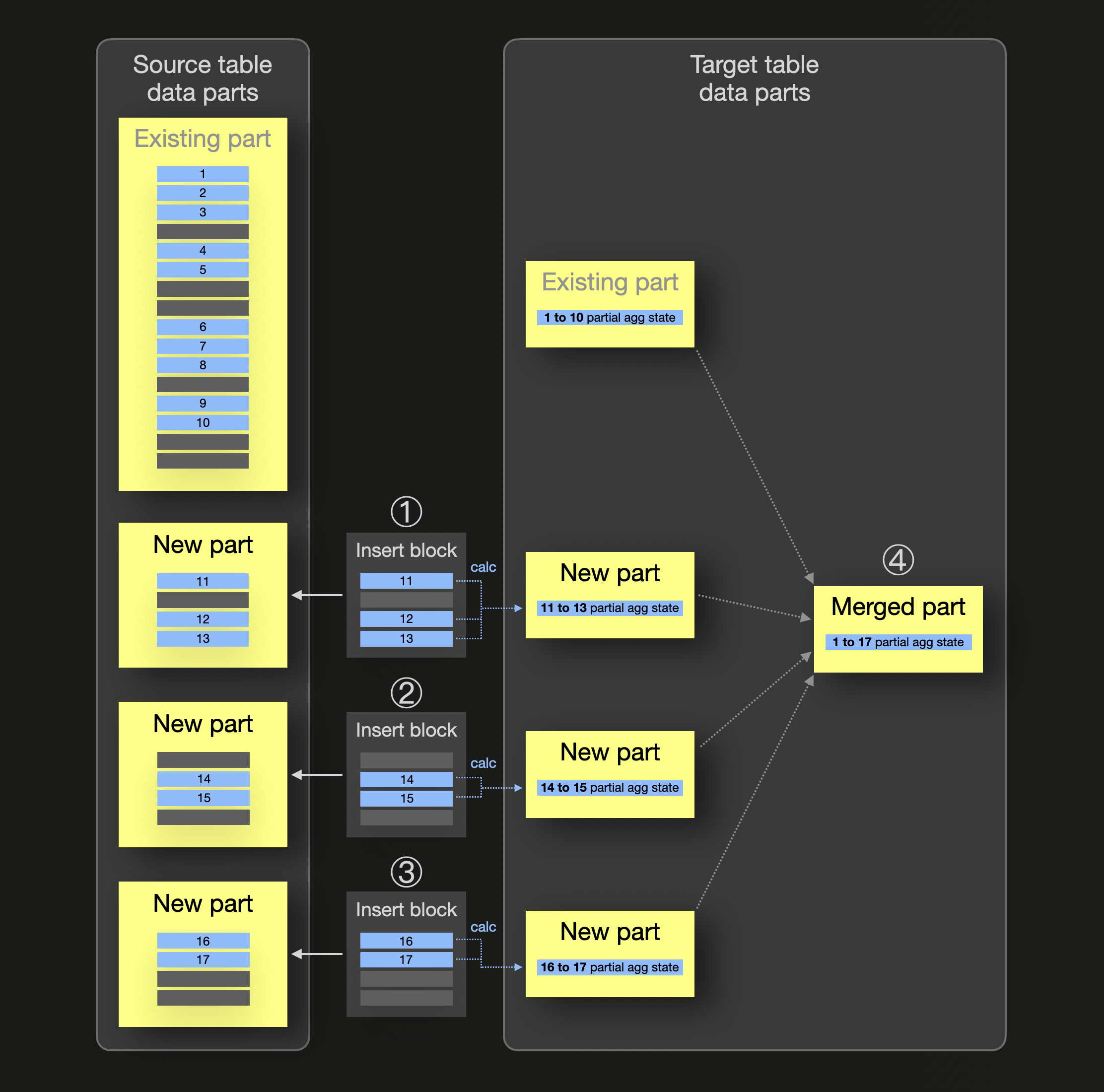
In the diagram above, the materialized view's source table already contains a data part storing some blue rows (1 to 10) belonging to the same group. For this group, there also already exists a data part in the view's target table storing a partial aggregation state for the blue group. When ① ② ③ inserts into the source table with new rows take place, a corresponding source table data part is created for each insert, and, in parallel, (just) for each block of newly inserted rows, a partial aggregation state is calculated and inserted in the form of a data part into the materialized view's target table. ④ During background part merges, the partial aggregation states are merged, resulting in incremental data aggregation.

Note that all over 90 aggregate functions, including their combination with aggregate function combinators, support partial aggregation states.

You can see a more concrete example of ClickHouse materializes views here.

The advantages of ClickHouse's approach include:

• Always-up-to-date aggregates: Materialized views are always in sync with the source table.
• No background jobs: Aggregation is pushed to insert time rather than query time.
• Better real-time performance: Ideal for observability workloads and real-time analytics where fresh aggregates are required instantly.
• Composable: Materialized views can be layered or joined with other views and tables for more complex query acceleration strategies.
• Different TTLs: Different TTL settings can be applied to the source table and target table of the materialized view.

This model is particularly powerful for observability use cases where users need to compute metrics such as per-minute error rates, latencies, or top-N breakdowns without scanning billions of raw records per query.

Lakehouse support

ClickHouse and Elasticsearch take fundamentally different approaches to lakehouse integration. ClickHouse is a fully-fledged query execution engine capable of executing queries over lakehouse formats such as Iceberg and Delta Lake. These formats rely on efficient querying of Parquet files, which ClickHouse fully supports. ClickHouse can read both Iceberg and Delta Lake tables directly, enabling seamless integration with modern data lake architectures.

In contrast, Elasticsearch is tightly coupled to its internal data format and Lucene-based storage engine. It cannot directly query lakehouse formats or Parquet files, limiting its ability to participate in modern data lake architectures. Elasticsearch requires data to be transformed and loaded into its proprietary format before it can be queried.

ClickHouse's lakehouse capabilities extend beyond just reading data:

• Data Catalog Integration: ClickHouse supports integration with data catalogs like Iceberg REST catalog and AWS Glue, enabling automatic discovery and access to tables in object storage.
• Object Storage Support: Native support for querying data residing in S3, GCS, and Azure Blob Storage without requiring data movement.
• Query Federation: Ability to correlate data across multiple sources, including lakehouse tables, traditional databases, and ClickHouse tables using external dictionaries and table functions.
• Incremental Loading: Support for continuous loading from lakehouse tables into local MergeTree tables, using features like S3Queue and ClickPipes.
• Performance Optimization: Distributed query execution over lakehouse data using cluster functions for improved performance.

These capabilities make ClickHouse a natural fit for organizations adopting lakehouse architectures, allowing them to leverage both the flexibility of data lakes and the performance of a columnar database.